Analyzing WDmodel

This document describes the output produced by the WDmodel package.

• Analysis

  • The fit
  • Spectral flux calibration errors
  • Hydrogen Balmer line diagnostics
  • Posterior distributions
  • Output files

Analysis

There’s many different outputs (ascii files, bintables, plots) that are produced by the WDmodel package. We’ll describe the plots first - it is a good idea to look at your data before using numbers from the analysis.

1. The fit:

All the plots are stored in <spec basename>_mcmc.pdf in the output directory that is printed as you run the WDmodel fitter (default: out/<object name>/<spec basename>/.

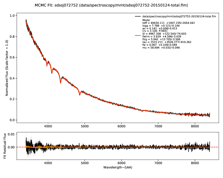
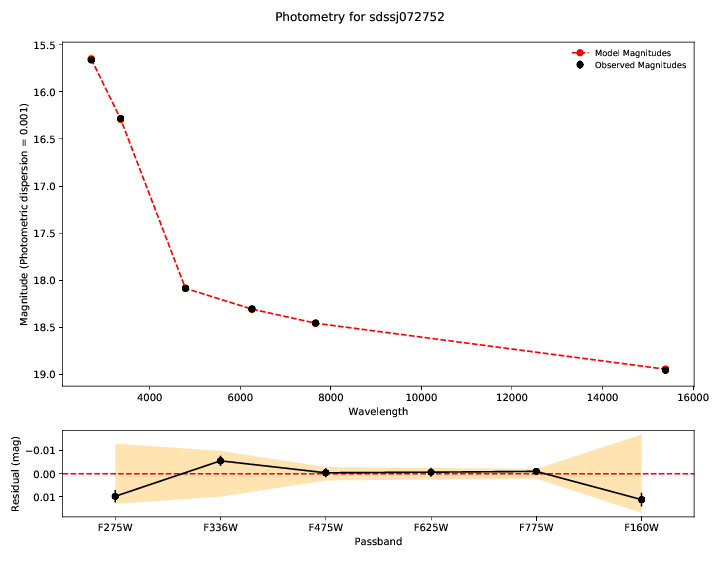
The first plots show you the bottom line - the fit of the model (red) to the data - the observed photometry and spectroscopy (black). Residuals for both are shown in the lower panel. The model parameters inferred from the data are shown in the legend of the spectrum plot. Draws from the posterior are shown in orange. The number of these is customizable with --ndraws. Observational uncertainties are shown as shaded grey regions.

If both of these don’t look reasonable, then the inferred parameters are probably meaningless. You should look at why the model is not in good agreement with the data. We’ve found this tends to happen if there’s a significant flux excess at some wavelengths, indicating a companion or perhaps variability.

2. Spectral flux calibration errors:

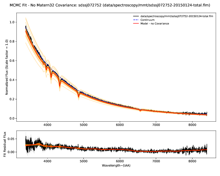
The WDmodel package uses a Gaussian process to model correlated flux calibration errors in the spectrum. These arise from a variety of sources (flat-fielding, background subtraction, extraction of the 2D spectrum with a polynomial, telluric feature removal, and flux calibration relative to some other spectrophotometric standard, which in turn is probably only good to a few percent). However, most of the processes that generate these errors would cause smooth and continuous deformations to the observed spectrum, and a single stationary covariance kernel is a useful and reasonable way to model the effects. The choice of kernel is customizable (--covtype, with default Matern32 which has proven more than sufficient for data from four different spectrographs with very different optical designs).

The residual plot shows the difference between the spectrum and best fit model without the Gaussian process applied. The residuals therefore show our estimate of the flux calibration errors and the Gaussian process model for them.

3. Hydrogen Balmer line diagnostics:

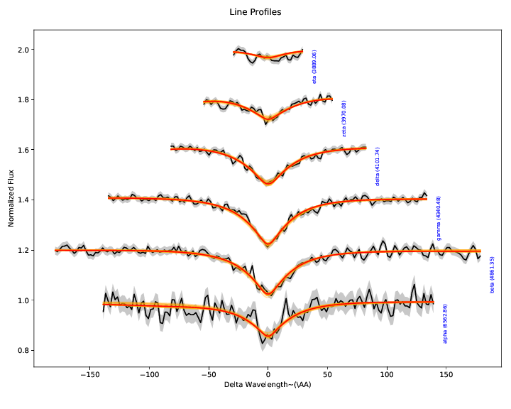
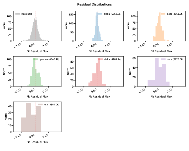
These plots illustrate the spectroscopic data and model specifically in the region of the Hydrogen Balmer lines. While the entire spectrum and all the photometry is fit simultaneously, we extract the Balmer lines, normalize their local continua to unity, and illustrate them separately here, offsetting each vertically a small amount for clarity.

With the exception of the SDSS autofit package used for their white dwarf analysis (which isn’t public in any case), every white dwarf atmosphere fitting code takes the approach of only fitting the Hydrogen Balmer lines to determine model parameters. This includes our own proof-of-concept analysis of Cycle 20 data. The argument goes that the inferred model parameters aren’t sensitive to reddening if the local continuum is divided out, and the line profiles determine the temperature and surface gravity.

In reality, reddening also changes the shape of the line profiles, and to divide out the local continuum, a model for it had to be fit (typically a straight line across the line from regions defined “outside” the line profile wings). The properties of this local continuum are strongly correlated with reddening, and errors in the local continuum affect the inference of the model parameters, particularly at low S/N. This is the regime our program to observe faint white dwarfs operates in - low S/N with higher reddening. Any reasonable analysis of systematic errors should illustrate significant bias resulting from the naive analysis in the presence of correlated errors.

In other words, the approach doesn’t avoid the problem, so much as shove it under a rug with the words “nuisance parameters” on top. This is why we adopted the more complex forward modeling approach in the WDmodel package. Unfortunately, Balmer profile fits are customary in the field, so after we forward model the data, we make a simple polynomial fit to the continuum (using our best understanding of what SDSS’ autofit does), and extract out the Balmer lines purely for this visualization. This way the polynomial continuum model does have no affect on the inference, and if it goes wrong and the Balmer line profile plots look wonky, it doesn’t actually matter.

If you mail the author about these plots, he will get annoyed and grumble about you, and probably reply with snark. He had no particular desire to even include these plots.

4. Posterior Distributions:

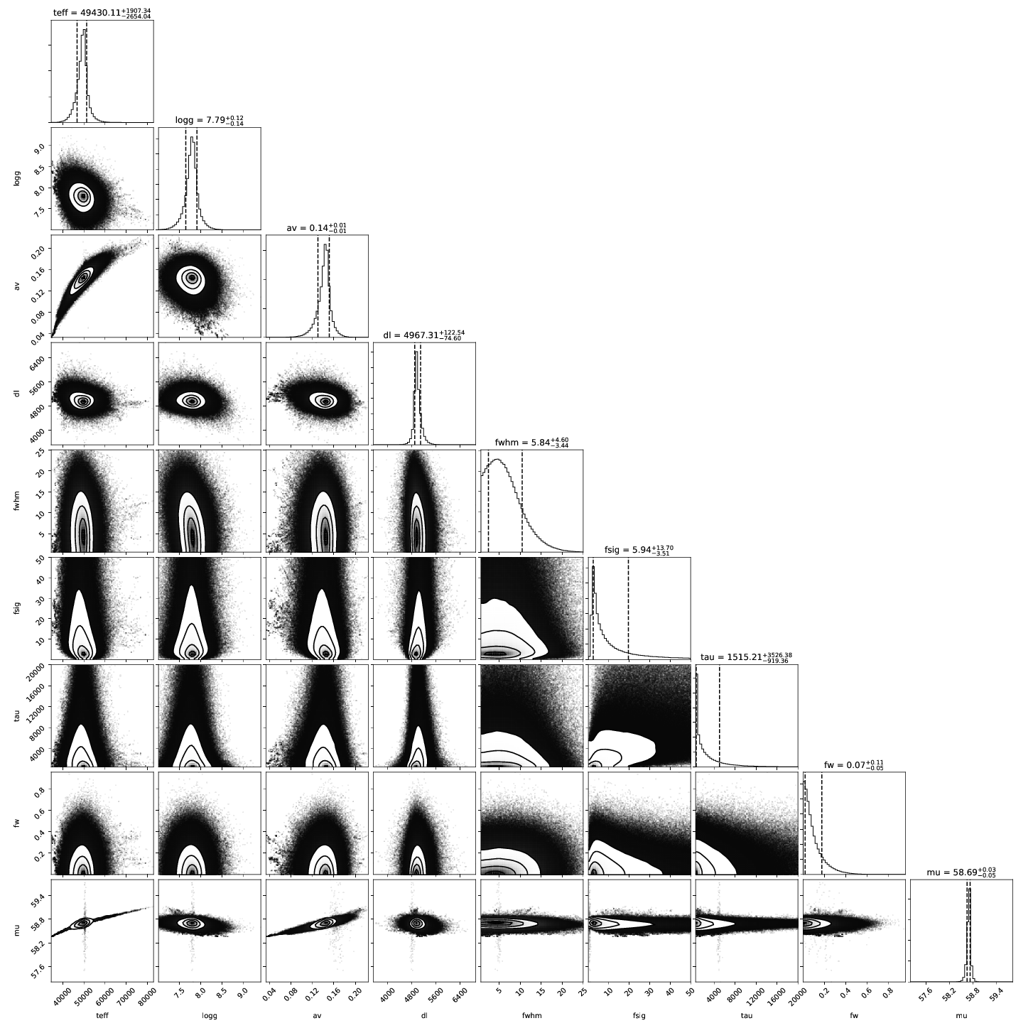
A corner plot of the posterior distribution. If the model and data are not in good agreement, then this is a good place to look. If you are running with --samptype=ensemble (the default), you might consider --samptype=pt --ntemps=5 --nwalkers=100 --nprod=5000 --thin 10 to better sample the posterior, and map out any multi-modality.

5. Output Files:

This table describes the output files produced by the fitter.

File	Description
<spec basename>_inputs.hdf5	All inputs to fitter and visualization module. Restored on --resume
<spec basename>_params.json	Initial guess parameters. Refined by minuit if not --skipminuit
<spec basename>_minuit.pdf	Plot of initial guess model, if refined by minuit
<spec basename>_mcmc.hdf5	Full Markov Chain - positions, log posterior, chain attributes
<spec basename>_mcmc.pdf	Plot of model and data after MCMC
<spec basename>_result.json	Summary of inferred model parameters, errors, uncertainties after MCMC
<spec basename>_spec_model.dat	Table of the observed spectrum and inferred model spectrum
<spec basename>_phot_model.dat	Table of the observed photometry and inferred model photometry
<spec basename>_full_model.hdf5	Derived normalized SED of the object

See Useful routines for some useful routines to summarize fit results.